The pack contains rubrics for the Maths AA SL course. There are scaffolds for basic and ambitious maths IAs. Rubrics that are student friendly and include example of how marks can be obtained. There is also a student checklist along with a comparison of the SL and HL IAs.

Based on the Pearson textbook there are 12 revision packs that have shorts exam questions with model answers and a GDC tips sheet. Each pack also has a section on what the IB usually asks.

This is a full scheme of work. Lesson by lesson with clear objectives, Key concepts and vocabulary, suggested activities, assessment and skills focus and a suggested video for flipped learning. It is split into 12 sections that follow the Pearson textbook. Each is a word document that can be amended or adapted for any of the textbooks. They work best with the study packs and Maths IA scaffolds and rubrics that are student friendly with examples that are needed for each possible mark in each section, that can also be downloaded.

Functions unit plan for IB Mathematics AA SL

Video explaining how to find the gradient of a line.

Unit 4 — Functions: Linear, Quadratic and Cubic Cambridge IGCSE 0607 Extended This unit develops students’ understanding of the three core function families and the algebraic techniques needed to manipulate, analyse and apply them. Students move from substitution and algebraic simplification through to recognising graphs by shape, finding key features using a GDC, and constructing equations from given information. The unit also introduces formal function language — domain, range, inverse and composite functions — and the effect of horizontal and vertical translations on a graph. By the end of the unit, students will be able to expand and factorise quadratic and cubic expressions, solve linear and quadratic equations (by factorisation, formula and GDC), solve simultaneous and quadratic inequalities, and find the equation of a quadratic from its vertex or intercepts. They will also be confident in using a GDC to sketch graphs, find zeros, locate maxima and minima, and identify points of intersection. The unit emphasises clear mathematical communication: showing every step of working, simplifying answers fully, using exact forms (such as surds or multiples of π\pi π) where required, and giving non-exact answers correct to at least three significant figures. Topics from this unit are assessed on the mid-course examination.

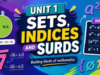
Unit 1 of 12. Unit 1 — Sets, Indices and Surds: Student Study Booklet A 30-page Cambridge IGCSE 0607 Extended study resource covering seven syllabus objectives: number types (E1.1), set notation and Venn diagrams (E1.2), squares/cubes/roots (E1.3), the rules of indices (E1.7), standard form (E1.8), surds and rationalising the denominator (E1.17), and equations involving indices (E2.4). Each section opens with a Learning Outcomes panel, builds the theory through numbered subsections with definitions, formulae and labelled diagrams, demonstrates technique through 2–3 worked examples, and closes with a 10-question bordered exercise. A complete Answer Section at the back provides fully worked solutions to all 70 questions, with every step of reasoning shown. All mathematics is typeset in LaTeX, and the booklet is presented to a professional standard suitable for distribution to students and parents. There is also a Calculator test and the unit description to accompany the notes booklet.

Unit 2 — Percentages and Equations: Student Study Booklet Cambridge IGCSE 0607 Extended | Number, Algebra and Functions This 49-page student study booklet provides comprehensive coverage of Unit 2 of the Cambridge IGCSE 0607 Extended syllabus, designed for direct distribution to students and parents. It mirrors the professional standard and visual style of the Unit 8 Mensuration booklet, with consistent typography, colour scheme, and layout throughout. Syllabus Coverage The booklet is divided into eleven numbered sections, each addressing one syllabus objective: C1.12 — Percentages (including deposits, discounts, profit and loss, simple and compound interest) C1.13 — Using a calculator efficiently and interpreting the display C1.15 — Calculating with money and currency conversion C2.1 — Letters as generalised numbers and substitution E2.2 — Simplifying expressions by collecting like terms C2.5 / E2.5 — Constructing and solving linear equations, simultaneous equations, and changing the subject of a formula C2.6 / E2.6 — Linear inequalities in one and two variables, including graphical regions E2.8 — Direct proportion (including y∝x2y \propto x^{2} y∝x2, x3x^{3} x3, and x\sqrt{x} x​) C3.1 / E3.1 — Linear functions and finding f(x)=ax+bf(x)=ax+b f(x)=ax+b from two points C3.2 — GDC skills with linear graphs (tables, intercepts, intersections, viewing windows) C3.3 / E3.3 — Function notation, domain and range, inverse and composite functions There is a Unit descriptor, Calculator and Non calculator test

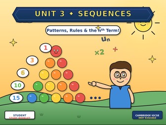
The main content is divided into eight numbered sections, each with its own clearly numbered subsections: Introduction to Sequences and Subscript Notation — defines a sequence, introduces unu_n un​ notation, distinguishes term-to-term from position-to-term rules. Continuing Sequences and Term-to-Term Rules — recognising and continuing patterns, including sequences with varying differences. Special Sequences — square, cube, and triangular numbers with their formulae and visual dot representations. Linear Sequences and the nn nth Term — finding un=an+bu_n = an + b un​=an+b, including a worked matchstick pattern problem. Quadratic Sequences and the nn nth Term — using second differences to find un=an2+bn+cu_n = an^2 + bn + c un​=an2+bn+c. Cubic Sequences and the nn nth Term — using third differences to find un=an3+bn2+cn+du_n = an^3 + bn^2 + cn + d un​=an3+bn2+cn+d. Exponential Sequences — geometric sequences with common ratio rr r, growth and decay, with a comparison chart. The Difference Method (Summary and Combinations) — consolidates all techniques into a single decision procedure and introduces combined sequences.

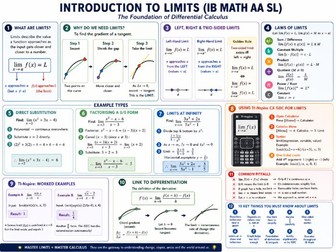
The PowerPoint introduces limits as the foundation of differential calculus for IB Mathematics AA SL. It explains why limits are needed to find the gradient of a tangent, beginning with secant gradients and then shrinking the gap so the secant approaches the tangent. It then defines a limit formally, covers one-sided and two-sided limits, and introduces the main limit laws. The presentation includes algebraic examples using direct substitution, factorising a 0/0 indeterminate form, and finding limits at infinity. It also shows how limits can be checked using the TI-Nspire CX GDC. The final section connects limits directly to differentiation through first principles:

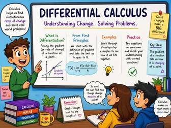
This presentation introduces students to the core idea of differential calculus by contrasting ordinary geometrical problems with calculus problems involving change, motion, and variation. It explains that calculus is needed when a quantity is not constant and we want to find an instantaneous rate of change, such as the gradient of a curve at a single point. The slides then develop differentiation from first principles, showing how the gradient of a secant becomes the gradient of a tangent as the interval gets smaller and smaller. Students are guided through worked examples step by step, before completing independent practice questions and checking their understanding with detailed worked answers. The overall aim is to build both conceptual understanding and procedural confidence in the foundations of differentiation.

Unit 5 — Trigonometry: Brief Summary Geometrical Vocabulary (C5.1) — Names and properties of angles, triangles, quadrilaterals, solids, and parts of a circle. Bearings (C5.2) — Three-figure angles measured clockwise from north. Back bearings differ by 180∘180^{\circ} 180∘. Pythagoras’ Theorem (C7.1) — a2+b2=c2a^2 + b^2 = c^2 a2+b2=c2 in right-angled triangles. Used for distances between points and chord-to-centre distances in circles. Right-Angled Trigonometry (C7.2) — SOH–CAH–TOA: sin⁡θ=opphyp\sin\theta = \tfrac{\text{opp}}{\text{hyp}} sinθ=hypopp​, cos⁡θ=adjhyp\cos\theta = \tfrac{\text{adj}}{\text{hyp}} cosθ=hypadj​, tan⁡θ=oppadj\tan\theta = \tfrac{\text{opp}}{\text{adj}} tanθ=adjopp​. Trigonometric Graphs (E3.1) — sin⁡x\sin x sinx and cos⁡x\cos x cosx have period 360∘360^{\circ} 360∘, amplitude 11 1; tan⁡x\tan x tanx has period 180∘180^{\circ} 180∘ with asymptotes. Elevation and Depression (E7.2) — Angles measured up or down from the horizontal; equal by alternate angles. Exact Values (E7.3) — Memorised values of sin⁡\sin sin, cos⁡\cos cos, tan⁡\tan tan at 0∘,30∘,45∘,60∘,90∘0^{\circ}, 30^{\circ}, 45^{\circ}, 60^{\circ}, 90^{\circ} 0∘,30∘,45∘,60∘,90∘. Trigonometric Equations (E7.4) — Solving sin⁡x=k\sin x = k sinx=k and cos⁡x=k\cos x = k cosx=k in [0∘,360∘][0^{\circ}, 360^{\circ}] [0∘,360∘] using graph symmetry. Sine and Cosine Rules (E7.5) — For any triangle: asin⁡A=bsin⁡B\tfrac{a}{\sin A} = \tfrac{b}{\sin B} sinAa​=sinBb​, a2=b2+c2−2bccos⁡Aa^2 = b^2 + c^2 - 2bc\cos A a2=b2+c2−2bccosA, Area =12absin⁡C= \tfrac{1}{2}ab\sin C =21​absinC. 3D Trigonometry (E7.6) — Extract right-angled triangles from solids; find space diagonals and angles between lines and planes. Chord Properties (E5.7) — Equal chords are equidistant from the centre; the perpendicular from the centre bisects a chord.

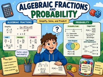
Section 1 — Arithmetic Fractions (C1.6) The four operations applied to fractions and mixed numbers. Use LCM to add/subtract; cancel and multiply by the reciprocal to divide. Section 2 — Core Algebraic Fractions (C2.3) The same rules applied to expressions with variables, where denominators are integers. Section 3 — Extended Algebraic Fractions (E2.3) Fractions with algebraic denominators. Factorise fully to simplify, and state any restrictions on the variable. Section 4 — Basic Probability (C9.1 / E9.1)The probability scale, the formula P(A)=favourabletotalP(A) = \frac{\text{favourable}}{\text{total}} P(A)=totalfavourable​, and the complement P(A′)=1−P(A)P(A’) = 1 - P(A) P(A′)=1−P(A). Section 5 — Relative Frequency and Expected Values (C9.2)Relative frequency estimates probability from experiments; expected frequency = P(event)×nP(\text{event}) \times n P(event)×n. Section 6 — Combined Events (C9.3 / E9.3) Three diagram methods — sample space, Venn, and tree diagrams — for calculating probabilities of combined and sequential events.

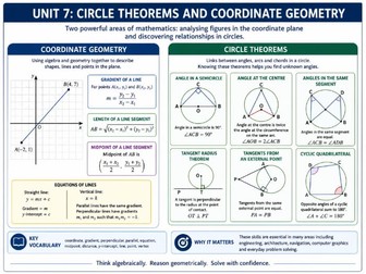
Unit 7 — Circle Theorems and Coordinate Geometry: Student Booklet A 48-page teaching pack for Cambridge IGCSE 0607 Extended Mathematics, designed to take students through the entire Unit 7 syllabus in a single self-contained resource. The booklet opens with a professionally designed title page and a navigable table of contents, followed by nine teaching sections that mirror the syllabus references: Cartesian coordinates, gradient, length and midpoint, the equation of a straight line, parallel and perpendicular lines, geometrical vocabulary, angle properties, and the two strands of circle theorems (Core, then Extended). Each section follows a consistent four-part structure — clear learning outcomes, theory presented with key ideas highlighted, fully worked examples, and an exercise of ten numbered questions for independent practice. The pack closes with Section 10, which contains complete step-by-step solutions to every one of the 90 exercise questions. Mathematical notation is written throughout in formal LaTeX, with proper angle notation, exact-form answers where appropriate, and clearly labelled diagrams illustrating each new concept. The booklet is suitable both for in-class teaching and for independent home study, and is presented to a standard appropriate for distribution to students and parents.

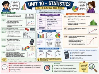
Unit 10 Statistics — Booklet Summary A 50-page study booklet for Cambridge IGCSE 0607 Extended, matching the Unit 8 Mensuration format. Structure: Eight sections, each with learning outcomes, notes, worked examples, and a 10-question exercise. Full worked solutions at the back. Sections: C10.1 — Tally charts, frequency tables, two-way tables C10.2 — Interpreting data; comparing sets using average + spread in context C10.3 — Discrete vs continuous data; class intervals C10.4 / E10.4 — Mean, median, mode, range, quartiles, IQR; estimated mean for grouped data C10.5 — GDC procedures (Casio and TI) for summary statistics C10.6 — Bar charts (simple, stacked, dual), pie charts, line graphs, pictograms, stem-and-leaf C10.7 / E10.7 — Scatter diagrams, correlation, line of best fit, linear regression E10.8 — Cumulative frequency curves; reading median, quartiles, percentiles Features: Custom TikZ diagrams throughout, proper LaTeX notation, GDC menu paths for both calculator brands, and 80 fully worked solutions. Test Calculator and Test Non-calculator

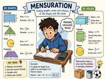
Unit 8 — Mensuration: Brief Summary The booklet covers eight syllabus objectives: C5.1 — Geometrical vocabulary: triangles, quadrilaterals, polygons, circles, solids, and bearings. C6.1 — Unit conversions for length, area, volume, capacity and mass, plus flow rates. C6.2 — Perimeter and area of rectangles, triangles, parallelograms and trapezia. C6.3 — Circumference, area, arc length and sector area, with answers in terms of π\pi π. C6.4 — Surface area and volume of cuboids, prisms, cylinders, cones, pyramids and spheres. C6.5 / E6.5 — Compound shapes, hollow solids and frustums. E5.3 — Similar shapes: linear, area and volume scale factors (kk k, k2k^2 k2, k3k^3 k3). E5.4 — Planes and axes of symmetry for common solids. Each section ends with a 10-question exercise, and full worked solutions appear at the back.

Unit 9 notes booklet. E2.4 Indices — Add indices when multiplying, subtract when dividing, multiply when raising a power to a power. a0=1a^0 = 1 a0=1, a−n=1/ana^{-n} = 1/a^n a−n=1/an, am/n=amna^{m/n} = \sqrt[n]{a^m} am/n=nam​. Solve ax=ba^x = b ax=b by writing both sides as the same base. E2.5 Equations & Subjects — Clear fractions by multiplying by the LCD. To change subject, isolate the term and undo in reverse order; if the new subject appears twice, collect, factorise, divide. E2.8 Proportion — Direct: y=kxy = kx y=kx. Inverse: y=k/xy = k/x y=k/x. Find kk k from a given pair, then use the equation. For inverse proportion, xy=kxy = k xy=k is constant. E3.1 Reciprocal & Exponential — y=a/x+by = a/x + b y=a/x+b has asymptote y=by = b y=b; y=a⋅bx+cy = a \cdot b^x + c y=a⋅bx+c has asymptote y=cy = c y=c. Two points pin down the parameters. E3.3 Functions — Domain = allowed inputs; range = actual outputs. Find f−1f^{-1} f−1 by swapping xx x and yy y then solving. f(g(x))f(g(x)) f(g(x)) applies gg g first, then ff f. 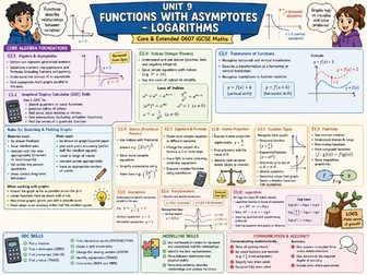E3.5 Asymptotes — Vertical: where the function blows up (denominator zero, log argument zero). Horizontal: the constant the curve approaches as x→±∞x \to \pm\infty x→±∞. E3.6 Transformations — f(x)+kf(x) + k f(x)+k shifts up by kk k; f(x−k)f(x - k) f(x−k) shifts right by kk k (sign flips!). Asymptotes move with the graph. E3.10 Logarithms — y=ax  ⟺  x=log⁡ayy = a^x \iff x = \log_a y y=ax⟺x=loga​y. Laws: log⁡(xy)=log⁡x+log⁡y\log(xy) = \log x + \log y log(xy)=logx+logy, log⁡(x/y)=log⁡x−log⁡y\log(x/y) = \log x - \log y log(x/y)=logx−logy, log⁡(xn)=nlog⁡x\log(x^n) = n \log x log(xn)=nlogx. Solve ax=ba^x = b ax=b by taking logs of both sides. Test calculator and Non-calculator.

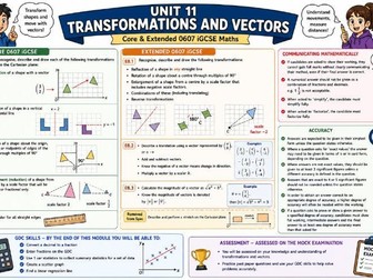
Unit 11 — Quick Summary Section 1 — Core Transformations Four types, each described by specific information. A translation slides a shape and is described by a column vector. A reflection flips a shape in a horizontal or vertical mirror line. A rotation turns a shape and needs a centre, an angle (a multiple of ninety degrees), and a direction. An enlargement resizes a shape from a centre by a scale factor; image lengths are the scale factor times the corresponding object lengths. Section 2 — Extended Transformations The mirror line for a reflection can now be any straight line, with the lines through the origin at forty-five degrees being especially common. A rotation can be about any centre, found by subtracting the centre, rotating about the origin, and adding the centre back. A negative scale factor inverts the image through the centre of enlargement. To reverse a combination of transformations, reverse each step and apply them in the opposite order. Section 3 — Vectors A vector has both magnitude and direction, and can be written as a column, as a directed line-segment between two points, or as a bold lowercase letter. Addition and subtraction are done component by component. The negative of a vector reverses its direction but keeps its magnitude. Multiplying by a scalar stretches the vector and reverses its direction if the scalar is negative. Two non-zero vectors are parallel exactly when one is a scalar multiple of the other. Section 4 — Magnitude The magnitude of a vector is its length, found by Pythagoras’ theorem on its two components. The magnitude of the vector from one point to another is simply the distance between those two points. Magnitudes should be given exactly in surd form where possible, otherwise to at least three significant figures.